A Practical Guide for Building Neural Networks using PyTorch

Deep Learning is a field of Artificial Intelligence (AI) where machines imitate the human brain and learn from their own experiences. In other words, machines can perform tasks requiring human intelligence. 

It is proliferating, and thousands of research papers are being published yearly. This research has given us advanced technologies like Face Detection, Chat Bots, Google Search, etc. 

There are a lot of libraries available for implementing Deep learning. One of them is PyTorch, developed by Facebook (currently Meta). 

In this article, we will talk about implementing Deep learning with PyTorch.

What is Deep Learning?

Often abbreviated as DL, it is an approach to learning a dataset by identifying its patterns. It is a subset of machine learning that learns from large amounts of data inspired by the human brain and neurons and makes accurate predictions. 

Basically, it is a neural network with three or more layers. Though a neural network with a single layer makes predictions, the depth of layers adds more accuracy to the predictions.  

Deep Learning is quite similar to how people learn from experience. Here, machines learn from their experiences and mimic human brains. 

The technology powers various everyday products, such as digital assistants, credit card fraud detection, self-driving cars, and voice-enabled TV remotes. 

What are Neural Networks? 

It is a system of algorithms aiming to find underlying patterns in a data set by mimicking the human brain. 

Neural networks in this context are systems of neurons through which input data "flows" before producing output. They can provide the optimal output by continuously iterating input data and minimizing the error between expected and actual output at each iteration. This task is performed until the algorithm is terminated or a global minimum is reached. 

Below is a high-level illustration of how neural networks operate. 

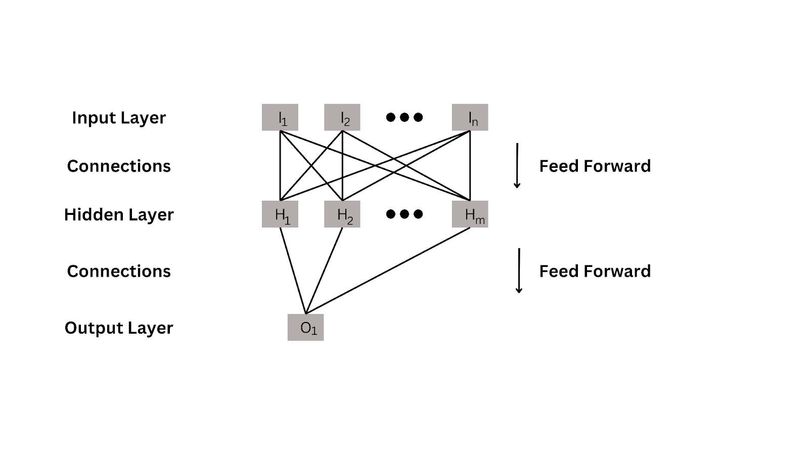
• In the above figure, the single input data is passed into the network. The input can be of any dimension. Primarily, 2D or 3D inputs are employed in the case of the image dataset. 

• Depending on the use case, the input data is passed through some mathematical activation function like sigmoid, tan, or RELU. This is mainly done to train the neuron to “activate” or “deactivate,” depending on the input data.

• After the propagation, an output is received at the outermost layer of the network. The expected output is then compared with the actual output using a loss function.

• Each neuron learns when to activate and deactivate by learning iteratively.

• Once the training is done, we can pass the real-world input data for which we need to predict the output.

Why is Deep Learning so Popular?

1. Feature Extraction

Each layer's ability to focus on mining a specific characteristic is one of the best features of DL. This is because it eliminates the need for human-made features, which are time-consuming and require significant experience and trial-and-error to get correct. 

With deep learning, you simply feed your model unprocessed data, and it will automatically extract the desired characteristics. This makes DL models extremely straightforward for individuals with limited statistical and domain knowledge in general.

2. Matrix Algebra

Many matrix calculations are involved in the training of Deep learning, which led to the development of Graphical Processing Units (GPUs). As linear algebra forms the base for DL, GPUs can perform most layer calculations in parallel. This enables the development of highly scalable, distributed models that provide greater accuracy at a much faster rate.

3. Train Massive Data sets without Overfitting.

You might think that more data means more accuracy of the model. However, statistics-based models cannot deal with vast amounts of data because of overfitting. 

Adding more layers enables deep learning to solve this problem simply. More layers result in more coefficients, making it more difficult to overfit. This allows you to train on gigabytes or even terabytes of data, which finally leads to improved performance.

ChatGPT is one example of a chatbot developed by OpenAI. The inception of ChatGPT has taken the world by storm. With this inception, another out-of-the-box invention is ChatBCG for converting text to slides. It eliminates the hustle of creating professional-looking PowerPoint presentations. 

What is PyTorch? 

Pytorch is a Python library that supports the development of computer vision and natural language processing applications. It emphasizes flexibility and allows simple Python code to represent DL models. 

This accessibility and user-friendly nature attracted early adopters in the research community. Since its initial release, it has become one of the most prominent deep-learning libraries for many applications. 

PyTorch offers a great introduction to deep learning, similar to what Python does for programming. In addition, the library has been demonstrated to be certified for use in professional settings for high-profile, real-world work. It is a good choice for teaching DL due to its simple syntax, streamlined API, and ease of debugging. 

If you are a beginner, learning this library is strongly suggested. 

Is PyTorch Open Source?

PyTorch is based on the Torch library, used for applications such as computer vision and natural language processing. The Torch library was originally developed by Meta AI and is now maintained by the Linux Foundation. It is open-source, free software distributed under a modified BSD license. 

You can contribute to the PyTorch source code through this repository.

Diving into the Implementation

To import PyTorch, you need the package “torch”. We will construct our model using a module called "nn" in the Torch library. We also load datasets using the torch.utils.data module. 

To enable GPU, we can add the following optional code

Now, we will create a dataset that we will use to train the model

“transforms.Compose” object is used to apply multiple data preprocessing transformations to the dataset. In this case, the transforms.ToTensor() function converts the images from their original format (PIL images) to PyTorch tensors and the transforms.Normalize((0.5,), (0.5,)) function normalizes the pixel values of the images to have a mean of 0.5 and a standard deviation of 0.5.

The next two lines of code are loading the MNIST dataset by creating train_dataset and test_dataset objects using the datasets. MNIST class. The root parameter specifies where the dataset should be saved, the training parameter specifies whether the data is for training or not, and the transform parameter specifies the preprocessing transformations to be applied to the data. The download=True is specified to download the dataset if it is not already downloaded.

The next two lines of code are creating train_loader and test_loader objects using the torch.utils.data.DataLoader class. These objects are used to load the data in batches, and the batch_size parameter is specifying the number of samples to be loaded in each batch.

The next task is to create a class of a Neural Network model. 

The __init__ method in this example is initializing the network by creating three fully connected layers using the nn.Linear module. The first layer will have 128 neurons, the second layer will have 64 neurons, and the third layer will have 10 neurons. Each layer represents a fully connected layer known as a dense layer.

The nn.ReLU() and nn.Softmax(dim=1) are nonlinear activation functions that represent the ReLU (Rectified Linear Unit) and Softmax, respectively. ReLU is used as an activation function in the hidden layers, and softmax is used as an activation function in the output layer.

The forward method in the above code defines the forward pass of the network, which takes an input x and applies a series of linear transformations, followed by non-linear activation functions, to the input x.

We now create an instance of the neural network model and train the model.

Now, we are defining the loss function and the optimizer. The nn.CrossEntropyLoss() function is used as the loss function here, a commonly used loss function for multi-class classification problems in Machine Learning. 

We are using the Adam optimizer to update the network's parameters while training and the lr argument specifies the learning rate while training. Later, we start the training of the network using 10 epochs.

The next task is to test the network.

Conclusion

Deep learning is one of the revolutionizing technologies that has eased human lives. As they can mimic human brains, they make accurate predictions. We hope you found this article helpful in understanding the technology and implementing it using PyTorch. To do so, we have used the ‘nn’ and torch.utils.data modules of PyTorch.